Построение гистограммы распределения
Содержание
Построение гистограммы распределения
Импорт данных из текста
Текст с данными каждого тестирования баланса внимания доступен для копирования при нажатии кнопки «Экспортировать данные», расположенной в конце страницы с результатами. Комбинации клавиш для копирования: Ctrl-A (выделить все) и Ctrl-C (копировать).
Создадим переменную с текстом. Краткое название s означает «string, строка». Поскольку этот текст занимает много строк, то мы ограничиваем его тройными кавычками.
s='''lps=[
11.516,0.365;
18.657,0.319;
26.752,0.313;
33.457,0.415;
40.614,0.379;
49.785,0.439;
58.077,0.436;
66.954,0.43;
73.462,0.411;
77.899,0.318;
81.582,0.331;
85.394,0.278;
89.357,0.259;
94.11,0.291;
98.307,0.333;
102.495,0.354;
107.003,0.373;
108.639,0.314;
110.709,0.308;
112.328,0.305;
114.396,0.309;
116.433,0.311;
118.837,0.323;
120.655,0.337;
131.162,0.47;
140.221,0.331;
147.681,0.312;
157.215,0.321;
164.737,0.416;
171.2,0.544;
178.674,0.287;
185.737,0.703;
192.244,0.372;
195.493,0.539;
199.887,0.29;
204.577,0.239;
209.183,0.289;
213.338,0.447;
216.879,0.45;
220.159,0.353;
224.665,0.399;
226.277,0.339;
228.446,0.282;
230.339,0.302;
232.707,0.31;
234.945,0.296;
236.729,0.287;
238.924,0.276]'''
len(s)
702
Длина текста - 702 символа. Мы видим, что одни символы означают нужные нам числа, а другие - разделители между числами. Для извлечения чисел мы можем использовать методы поиска подстроки для очистки текста от ненужных символов, а для конвертации в числовой массив - специальные команды для создания массивов.
#найдем квадратные скобки, ограничивающие данные
iab=s.find('[')
iad=s.find(']')
s=s[iab:iad+1]  #оставляем только то, что между скобками
if len(s)>10:  #если между скобками что-то есть
    a=array(mat(s.replace('\n','')))  #создаем массив (array)
else:    #иначе заведем пустой массив (на случай неверных исходных данных)
    a=array([])
a.shape
(48, 2)
Форма полученного массива чисел - 48 на 2, то есть 48 строк и 2 колонки.
Просмотрите содержимое переменной
a(создайте ячейку, вставьте туда название переменной и выполните).
Импорт данных с веб-странички
Когда Вы просматриваете страницу результатов теста в браузере, то видите результаты обработки данных в виде рисунков и прочего. Следовательно, в составе информации, которую получил браузер в ответ на запрос к серверу, присутствуют нужные нам данные. Надо лишь извлечь их!
Исходный код веб-страницы можно посмотреть, нажав Ctrl-U (или пункт меню «Посмотреть код страницы» или «Исходный код страницы»).
Внутри одного из тегов <script type="text/javascript"> (скрипте на языке JavaScript) задается переменная с данными, на основании которых строятся рисунки. Вы можете найти строку, начинающуюся на lps= (Для поиска на странице нажмите Ctrl-F) следующего формата:
lps=[[9.585,0.429], [16.368,0.335], [23.729,0.357], ...
Это как раз те данные, что нам нужны. Значение переменной представляет собой описание массива, состоящего из множества маленьких массивчиков, в каждом из которых по два значения.
Библиотека urllib позволяет работать с URL как с файлами, т.е. открыть их и прочитать содержимое.
import urllib

u = 'http://balatte.stireac.com/balatte/result/ntkharchenko%40mail.ru/up9.valeo.sfedu.ru__20111212T135308671'
s = urllib.request.urlopen(u).read()
print ('Скачано {} байт!'.format(len(s)))
Скачано 8563 байт!
Если Вы посмотрите содержимое переменной s, то увидите запутанный HTML код - тот же, что мы видели в браузере через пункт меню «Посмотреть исходный код».
Для нахождения нужного нам фрагмента по характерным символам в его начале и конце используем библиотеку re для работы с регулярными выражениями (regular expressions).
import re

s = str(s)   # преобразуем скачанные байты в строку
m = re.search(r'lps=(\[\[.+?\]\])',s)
a = array(eval(m.group(1)))
a.shape
(45, 2)
Функция eval() выполняет команды в передаваемом ей тексте, т.е. воспринимает текст как программный код. Безошибочность данной операции обеспечивается за счет сходства синтаксиса построения массивов в языках Python и JavaScript.
Мы познакомились с несколькими вариантами извлечения данных из открытых ресурсов.
В случае с данными из теста на внимание в итоге мы получили двумерный массив чисел, первая колонка - время предъявления стимулов, с; вторая колонка - время реакции (латентный период), с.
Гистограмма
Теперь, когда мы разобрались со структурой наших данных,
берем значения из второй колонки и строим гистограмму распределения с помощью функции hist.
Вторая колонка имеет индекс 1, поскольку индексация начинается с 0, и 0 - это первая по счёту колонка.
vv = a[:,1]
hist(vv)
(array([ 9.,  6., 15.,  8.,  2.,  3.,  0.,  0.,  1.,  1.]),
 array([0.282 , 0.3236, 0.3652, 0.4068, 0.4484, 0.49  , 0.5316, 0.5732,
        0.6148, 0.6564, 0.698 ]),
 <BarContainer object of 10 artists>)
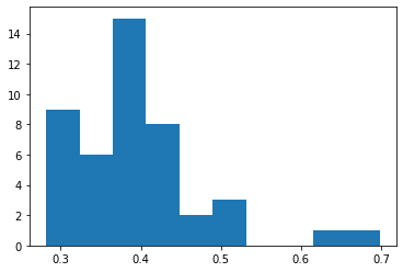
По информации, возвращаемой функцией hist, ясно, что значения были разделены на 10 групп. Границы групп идут с равным шагом от 0.2 до 0.7, что видно по оси абсцисс.
По оси ординат отложено количество значений в каждой группе.
Чтобы не гадать, что за информация возвращается функцией hist, обратимся к документации.
hist?
Signature:
hist(
    x,
    bins=None,
    range=None,
    density=False,
    weights=None,
    cumulative=False,
    bottom=None,
    histtype='bar',
    align='mid',
    orientation='vertical',
    rwidth=None,
    log=False,
    color=None,
    label=None,
    stacked=False,
    *,
    data=None,
    **kwargs,
)
Docstring:
Plot a histogram.

Compute and draw the histogram of *x*.  The return value is a tuple
(*n*, *bins*, *patches*) or ([*n0*, *n1*, ...], *bins*, [*patches0*,
*patches1*, ...]) if the input contains multiple data.  See the
documentation of the *weights* parameter to draw a histogram of
already-binned data.

Multiple data can be provided via *x* as a list of datasets
of potentially different length ([*x0*, *x1*, ...]), or as
a 2-D ndarray in which each column is a dataset.  Note that
the ndarray form is transposed relative to the list form.

Masked arrays are not supported.

The *bins*, *range*, *weights*, and *density* parameters behave as in
`numpy.histogram`.

Parameters
----------
x : (n,) array or sequence of (n,) arrays
    Input values, this takes either a single array or a sequence of
    arrays which are not required to be of the same length.

bins : int or sequence or str, default: :rc:`hist.bins`
    If *bins* is an integer, it defines the number of equal-width bins
    in the range.

    If *bins* is a sequence, it defines the bin edges, including the
    left edge of the first bin and the right edge of the last bin;
    in this case, bins may be unequally spaced.  All but the last
    (righthand-most) bin is half-open.  In other words, if *bins* is::

        [1, 2, 3, 4]

    then the first bin is ``[1, 2)`` (including 1, but excluding 2) and
    the second ``[2, 3)``.  The last bin, however, is ``[3, 4]``, which
    *includes* 4.

    If *bins* is a string, it is one of the binning strategies
    supported by `numpy.histogram_bin_edges`: 'auto', 'fd', 'doane',
    'scott', 'stone', 'rice', 'sturges', or 'sqrt'.

range : tuple or None, default: None
    The lower and upper range of the bins. Lower and upper outliers
    are ignored. If not provided, *range* is ``(x.min(), x.max())``.
    Range has no effect if *bins* is a sequence.

    If *bins* is a sequence or *range* is specified, autoscaling
    is based on the specified bin range instead of the
    range of x.

density : bool, default: False
    If ``True``, draw and return a probability density: each bin
    will display the bin's raw count divided by the total number of
    counts *and the bin width*
    (``density = counts / (sum(counts) * np.diff(bins))``),
    so that the area under the histogram integrates to 1
    (``np.sum(density * np.diff(bins)) == 1``).

    If *stacked* is also ``True``, the sum of the histograms is
    normalized to 1.

weights : (n,) array-like or None, default: None
    An array of weights, of the same shape as *x*.  Each value in
    *x* only contributes its associated weight towards the bin count
    (instead of 1).  If *density* is ``True``, the weights are
    normalized, so that the integral of the density over the range
    remains 1.

    This parameter can be used to draw a histogram of data that has
    already been binned, e.g. using `numpy.histogram` (by treating each
    bin as a single point with a weight equal to its count) ::

        counts, bins = np.histogram(data)
        plt.hist(bins[:-1], bins, weights=counts)

    (or you may alternatively use `~.bar()`).

cumulative : bool or -1, default: False
    If ``True``, then a histogram is computed where each bin gives the
    counts in that bin plus all bins for smaller values. The last bin
    gives the total number of datapoints.

    If *density* is also ``True`` then the histogram is normalized such
    that the last bin equals 1.

    If *cumulative* is a number less than 0 (e.g., -1), the direction
    of accumulation is reversed.  In this case, if *density* is also
    ``True``, then the histogram is normalized such that the first bin
    equals 1.

bottom : array-like, scalar, or None, default: None
    Location of the bottom of each bin, ie. bins are drawn from
    ``bottom`` to ``bottom + hist(x, bins)`` If a scalar, the bottom
    of each bin is shifted by the same amount. If an array, each bin
    is shifted independently and the length of bottom must match the
    number of bins. If None, defaults to 0.

histtype : {'bar', 'barstacked', 'step', 'stepfilled'}, default: 'bar'
    The type of histogram to draw.

    - 'bar' is a traditional bar-type histogram.  If multiple data
      are given the bars are arranged side by side.
    - 'barstacked' is a bar-type histogram where multiple
      data are stacked on top of each other.
    - 'step' generates a lineplot that is by default unfilled.
    - 'stepfilled' generates a lineplot that is by default filled.

align : {'left', 'mid', 'right'}, default: 'mid'
    The horizontal alignment of the histogram bars.

    - 'left': bars are centered on the left bin edges.
    - 'mid': bars are centered between the bin edges.
    - 'right': bars are centered on the right bin edges.

orientation : {'vertical', 'horizontal'}, default: 'vertical'
    If 'horizontal', `~.Axes.barh` will be used for bar-type histograms
    and the *bottom* kwarg will be the left edges.

rwidth : float or None, default: None
    The relative width of the bars as a fraction of the bin width.  If
    ``None``, automatically compute the width.

    Ignored if *histtype* is 'step' or 'stepfilled'.

log : bool, default: False
    If ``True``, the histogram axis will be set to a log scale. If
    *log* is ``True`` and *x* is a 1D array, empty bins will be
    filtered out and only the non-empty ``(n, bins, patches)``
    will be returned.

color : color or array-like of colors or None, default: None
    Color or sequence of colors, one per dataset.  Default (``None``)
    uses the standard line color sequence.

label : str or None, default: None
    String, or sequence of strings to match multiple datasets.  Bar
    charts yield multiple patches per dataset, but only the first gets
    the label, so that `~.Axes.legend` will work as expected.

stacked : bool, default: False
    If ``True``, multiple data are stacked on top of each other If
    ``False`` multiple data are arranged side by side if histtype is
    'bar' or on top of each other if histtype is 'step'

Returns
-------
n : array or list of arrays
    The values of the histogram bins. See *density* and *weights* for a
    description of the possible semantics.  If input *x* is an array,
    then this is an array of length *nbins*. If input is a sequence of
    arrays ``[data1, data2, ...]``, then this is a list of arrays with
    the values of the histograms for each of the arrays in the same
    order.  The dtype of the array *n* (or of its element arrays) will
    always be float even if no weighting or normalization is used.

bins : array
    The edges of the bins. Length nbins + 1 (nbins left edges and right
    edge of last bin).  Always a single array even when multiple data
    sets are passed in.

patches : `.BarContainer` or list of a single `.Polygon` or list of such objects
    Container of individual artists used to create the histogram
    or list of such containers if there are multiple input datasets.

Other Parameters
----------------
**kwargs
    `~matplotlib.patches.Patch` properties

See Also
--------
hist2d : 2D histograms

Notes
-----
For large numbers of bins (>1000), 'step' and 'stepfilled' can be
significantly faster than 'bar' and 'barstacked'.

.. note::
    In addition to the above described arguments, this function can take
    a *data* keyword argument. If such a *data* argument is given,
    the following arguments can also be string ``s``, which is
    interpreted as ``data[s]`` (unless this raises an exception):
    *x*, *weights*.

    Objects passed as **data** must support item access (``data[s]``) and
    membership test (``s in data``).
File:      c:\a\winpython\python-3.9.0rc1.amd64\lib\site-packages\matplotlib\pyplot.py
Type:      function
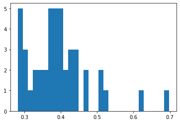
Важный параметр - bins (корзинки, ячейки, ящички) - определенное число заданных интервалов, попадание в которые подсчитывается. Можно задать в штуках, а можно в виде перечня границ. Интервалы обычно делают одинаковой ширины, хотя это не обязательно.
hist(vv, bins=30);
Количество/ширину интервалов обычно подбирают на глаз. Поскольку обычно стоит задача оценить форму распределения, то автоматические методы подбора «оптимального» количества классов опираются на характеристики распределения - моменты распределения:
Среднее (mean)
Дисперсия (variance, вариация)
Асимметричность (skewness, скошенность, неравенство хвостов)
Эксцесс (kurtosis, тяжесть хвостов)
from scipy.stats import kurtosis, skew
sturges = lambda data: int(log2(len(data)) + 1)
rice = lambda data: int(2*len(data)**0.333)
wichard = lambda data: int(1 + log2(len(data)) + log2(1 + kurtosis(data) * (len(data) / 6.) ** 0.5))
doane = lambda data: int(1 + log2(len(data)) + log2(1 + abs(skew(data))/(6*(len(data)-2)/((len(data)+1)*(len(data)+3)))**0.5 ))
vv = vv[~isnan(vv)] # удалим пропущенные значения
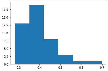
sturges(vv), rice(vv), doane(vv), wichard(vv)
(6, 7, 8, 9)
Ссылки на описания методов.
Sturges, H.A. (1926). «The choice of a class interval». Journal of the American Statistical Association: 65–66. doi:10.1080/01621459.1926.10502161.
Lane D.M. (2007) http://onlinestatbook.com/2/graphing_distributions/histograms.html
Doane D.P. (1976) Aesthetic frequency classification. American Statistician, 30: 181–183
Wichard J. D., Kuhne R., Ter Laak A. Binding site detection via mutual information //2008 IEEE International Conference on Fuzzy Systems (IEEE World Congress on Computational Intelligence). – IEEE, 2008. – С. 1770-1776.
hist(vv, bins=6);
Другой полезный параметр - density (плотность), который позволяет нормировать высоту столбцов в процентах к общему числу данных.
В результате получается эмпирическая плотность вероятности: т.е. чем выше столбик в этом месте диапазона, тем больше вероятность, что значения попадают в данный интервал.
В этой же шкале мы можем наложить теоретическое нормальное распределение (и любое другое).
import scipy.stats as stats

hist(vv, density=True, label='данные')

#найдем характеристики распределения (предположительно нормального)
M = mean(vv); S = std(vv);
xx = arange(0, 1, 0.01) #подробные значения абсцисс для гладкой кривой
yy = stats.norm.pdf(xx, M, S)
plot(xx, yy, 'r-', label='модель'); legend(); xlabel('ВР, с'); ylabel('%');
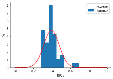
При наложении графиков эмпирического и теоретического распределений видно, что распределение значений времени реакций несимметричное.